Linear Discriminant Analysis for Starters
Linear discriminant analysis (commonly abbreviated to LDA, and not to be confused with the other LDA) is a very common dimensionality reduction technique for classification problems. However, that’s something of an understatement: it does so much more than “just” dimensionality reduction.
In plain English, if you have high-dimensional data (i.e. a large number of features) from which you wish to classify observations, LDA will help you transform your data so as to make the classes as distinct as possible. More rigorously, LDA will find the linear projection of your data into a lower-dimensional subspace that optimizes some measure of class separation. The dimension of this subspace is necessarily strictly less than the number of classes.
This separation-maximizing property of LDA makes it so good at its job that it’s sometimes considered a classification algorithm in and of itself, which leads to some confusion. Linear discriminant analysis is a form of dimensionality reduction, but with a few extra assumptions, it can be turned into a classifier. (Avoiding these assumptions gives its relative, quadratic discriminant analysis, but more on that later). Somewhat confusingly, some authors call the dimensionality reduction technique “discriminant analysis”, and only prepend the “linear” once we begin classifying. I actually like this naming convention more (it tracks the mathematical assumptions a bit better, I think), but most people nowadays call the entire technique “LDA”, so that’s what I’ll call it.
The goal of this post is to give a comprehensive introduction to, and explanation of, LDA. I’ll look at LDA in three ways:
- LDA as an algorithm: what does it do, and how does it do it?
- LDA as a theorem: a mathematical derivation of LDA
- LDA as a machine learning technique: practical considerations when using LDA
This is a lot for one post, but my hope is that there’s something in here for everyone.
Contents
LDA as an Algorithm
Problem statement
Before we dive into LDA, it’s good to get an intuitive grasp of what LDA tries to accomplish.
Suppose that:
- You have very high-dimensional data, and that
- You are dealing with a classification problem
This could mean that the number of features is greater than the number of observations, or it could mean that you suspect there are noisy features that contain little information, or anything in between.
Given that this is the problem at hand, you wish to accomplish two things:
- Reduce the number of features (i.e. reduce the dimensionality of your feature space), and
- Preserve (or even increase!) the “distinguishability” of your classes or the “separatedness” of the classes in your feature space.
This is the problem that LDA attempts to solve. It should be fairly obvious why this problem might be worth solving.
To judiciously appropriate a term from signal processing, we are interested in increasing the signal-to-noise ratio of our data, by both extracting or synthesizing features that are useful in classifying our data (amplifying our signal), and throwing out the features that are not as useful (attenuating our noise).
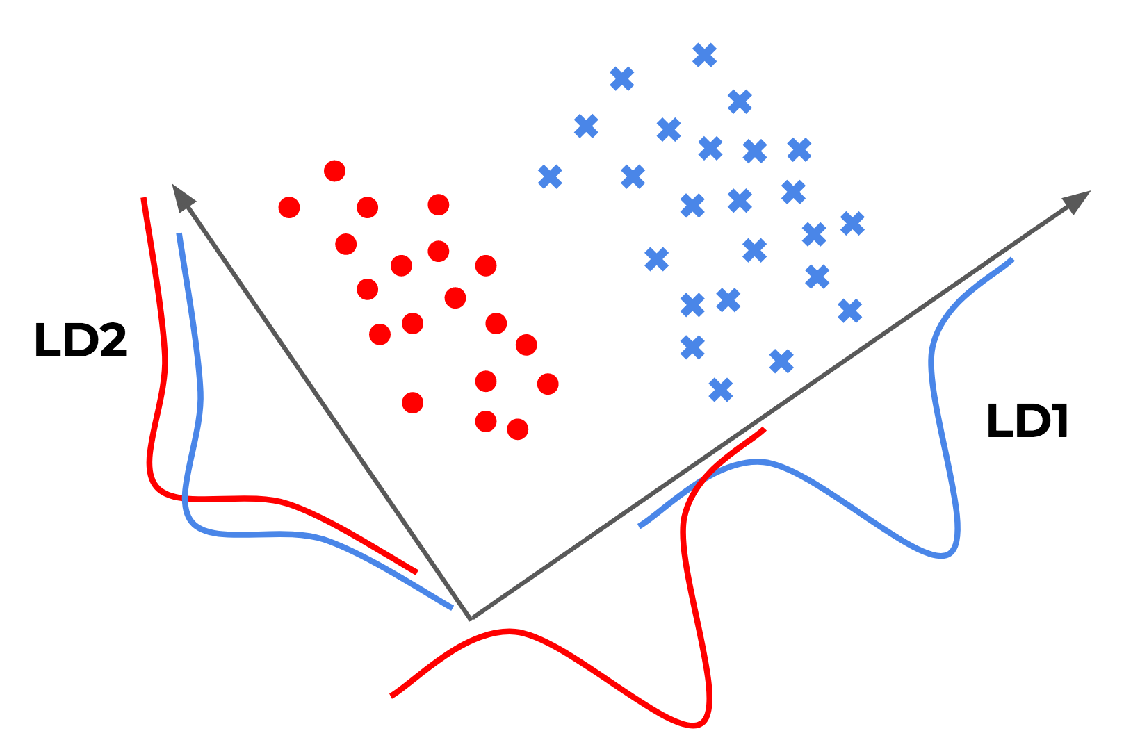
Below is simple illustration I made, inspired by Sebastian Raschka that may help our intuition about the problem:
A couple of points to make:
- LD1 and LD2 are among the projections that LDA would consider. In reality, LDA would consider all possible projections, not just those along the x and y axes.
- LD1 is the one that LDA would actually come up with: this projection gives the best “separation” of the two classes.
- LD2 is a horrible projection by this metric: both classes get horribly overlapped… (this actually relates to PCA, but more on that later)
UPDATE: For another illustration, Rahul Sangole made a simple but great interactive visualization of LDA here using Shiny.
Solution
First, some definitions:
Let:
- $n$ be the number of classes
- $\mu$ be the mean of all observations
- $N_i$ be the number of observations in the $i$th class
- $\mu_i$ be the mean of the $i$th class
- $\Sigma_i$ be the scatter matrix of the $i$th class
Now, define $S_W$ to be the within-class scatter matrix, given by
$$ \begin{align*} S_W = \sum_{i=1}^{n}{\Sigma_i} \end{align*} $$
and define $S_B$ to be the between-class scatter matrix, given by
$$ \begin{align*} S_B = \sum_{i=1}^{n}{N_i (\mu_i - \mu) (\mu_i - \mu)^T} \end{align*} $$
Diagonalize $S_W^{-1} S_B$ to get its eigenvalues and eigenvectors.
Pick the $k$ largest eigenvalues, and their associated eigenvectors. We will project our observations onto the subspace spanned by these vectors.
Concretely, what this means is that we form the matrix $A$, whose columns are the $k$ eigenvectors chosen above. $W$ will allow us to transform our observations into the new subspace via the equation $y = A^T x$, where $y$ is our transformed observation, and $x$ is our original observation.
And that’s it!
For a more detailed and intuitive explanation of the LDA “recipe”, see Sebastian Raschka’s blog post on LDA.
LDA as a Theorem
Sketch of Derivation:
In order to maximize class separability, we need some way of measuring it as a number. This number should be bigger when the between-class scatter is bigger, and smaller when the within-class scatter is larger. There are many such formulas/numbers that have this property: Fukunaga’s Introduction to Statistical Pattern Recognition considers no less than four! Here, we’ll concern ourselves with just one:
$$ J_1 = tr(S_{WY}^{-1} S_{BY}) $$
where I denote the within and between-class scatter matrices of the projection vector $Y$ by $S_{WY}$ and $S_{BY}$, to avoid confusion with the corresponding matrices for the projected vector $X$.
Now, a standard result from probability is that for any random variable $X$ and matrix $A$, we have $cov(A^T X) = A^T cov(X) A$. We’ll apply this result to our projection $y = A^T x$. It follows that
$$ S_{WY} = A^T S_{WX} A $$
and
$$ S_{BY} = A^T S_{BX} A $$
where $S_{BX}$ and $S_{BY}$ are the between-class scatter matrices, and $S_{WX}$ and $S_{WY}$ are the within-class scatter matrices, for $X$ and its projection $Y$, respectively.
It’s now a simple matter to write $J_1$ in terms of $A$, and maximize $J_1$. Without going into the details, we set $\frac{\partial J_1}{\partial A} = 0$ (whatever that means), and use the fact that the trace of a matrix is the sum of its eigenvalues.
I don’t want to go into the weeds with this here, but if you really want to see the algebra, Fukunaga is a great resource. The end result, however, is the same condition on the eigenvalues and eigenvectors as stated above: in other words, the optimization gives us LDA as presented.
There’s one more quirk of LDA that’s very much worth knowing. Suppose you have 10 classes, and you run LDA. It turns out that the maximum number of features LDA can give you is one less than the number of class, so in this case, 9!
Proposition: $S_W^{-1} S_B$ has at most $n-1$ non-zero eigenvalues, which implies that LDA is must reduce the dimension to at least $n-1$.
To prove this, we first need a lemma.
Lemma: Suppose ${v_i}{i=1}^{n}$ is a set of linearly dependent vectors, and let $\alpha_i$ be $n$ coefficients. Then, $M = \sum{i=1}^{n}{\alpha_i v_i v_i^{T}}$, a linear combination of outer products of the vectors with themselves, is rank deficient.
Proof: The row space of $M$ is generated by the set of vectors ${v_1, v_2, …, v_n}$. However, because this set of vectors is linearly dependent, it must span a vector space of dimension strictly less than $n$, or in other words less than or equal to $n-1$. But the dimension of the row space is precisely the rank of the matrix $M$. Thus, $rank(M) \leq n-1$, as desired.
With the lemma, we’re now ready to prove our proposition.
Proof: We have that
$$ \begin{align*} \frac{1}{n} \sum_{i=1}^{n}{\mu_i} = \mu \implies \sum_{i=1}^{n}{\mu_i-\mu} = 0 \end{align*} $$
So ${\mu_i-\mu}_{i=1}^{n}$ is a linearly dependent set. Applying our lemma, we see that
$$ S_B = \sum_{i=1}^{n}{N_i (\mu_i-\mu)(\mu_i-\mu)^{T}} $$
must be rank deficient. Thus, $rank(S_W) \leq n-1$. Now, $rank(AB) \leq rank(A)rank(B)$, so
$$ \begin{align*} rank(S_W^{-1}S_B) \leq \min{(rank(S_W^{-1}), rank(S_B))} = n-1 \end{align*} $$
as desired.
LDA as a Machine Learning Technique
OK so we’re done with the math, but how is LDA actually used in practice? One of
the easiest ways is to look at how LDA is actually implemented in the real
world. scikit-learn has a very well-documented implementation of
LDA:
I find that reading the docs is a great way to learn stuff.
Below are a few miscellaneous comments on practical considerations when using LDA.
Regularization (a.k.a. shrinkage)
scikit-learn’s implementation of LDA has an interesting optional parameter:
shrinkage. What’s that about?
Here’s a wonderful Cross Validated post on how LDA can introduce overfitting. In essence, matrix inversion is an extremely sensitive operation (in that small changes in the matrix may lead to large changes in its inverse, so that even a tiny bit of noise will be amplified upon inverting the matrix), and so unless the estimate of the within-class scatter matrix $S_W$ is very good, its inversion is likely to introduce overfitting.
One way to combat that is through regularizing LDA. It basically replaces
$S_W$ with $(1-t)S_W + tI$, where $I$ is the identity matrix, and $t$ is
the regularization parameter, or the shrinkage constant. That’s what
scikit’s shrinkage parameter is: it’s $t$.
If you’re interested in why this linear combination of the within-class scatter and the identity give such a well-conditioned estimate of $S_W$, check out the original paper by Ledoit and Wolf. Their original motivation was in financial portfolio optimization, so they’ve also authored several other papers (here and here) that go into the more financial details. That needn’t concern us though: covariance matrices are literally everywhere.
For an illustration of this, amoeba’s post on Cross Validated gives a good
example of LDA overfitting, and how regularization can help combat that.
LDA as a classifier
We’ve talked a lot about how LDA is a dimensionality reduction technique. But in addition to it, you can make two extra assumptions, and LDA becomes a very robust classifier as well! Here they are:
- Assume that the class conditional distributions are Gaussian, and
- Assume that these Gaussians have the same covariance matrix (a.k.a. assume homoskedasticity)
Now, how LDA acts as a classifier is a bit complicated: the problem is solved fairly easily if there are only two classes. In this case, the optimal Bayesian solution is to classify the observation depending on whether the log of the likelihood ratio is less than or greater than some threshold. This turns out to be a simple dot product: $\vec{w} \cdot \vec{x} > c$, where $\vec{w} = \Sigma^{-1} (\vec{\mu_1} - \vec{\mu_2})$. Wikipedia has a good derivation of this.
There isn’t really a nice dot-product solution for the multiclass case. So, what’s commonly done is to take a “one-against-the-rest” approach, in which there are $k$ binary classifiers, one for each of the $k$ classes. Another common technique is to take a pairwise approach, in which there are $k(k-1)/2$ classifiers, one for each pair of classes. In either case, the outputs of all the classifiers are combined in some way to give the final classification.
Close relatives: PCA, QDA, ANOVA
LDA is similar to a lot of other techniques, and the fact that they all go by acronyms doesn’t do anyone a favor. My goal here isn’t to introduce or explain these various techniques, but rather point out their differences.
1) Principal components analysis (PCA):
LDA is very similar to PCA: in fact, the question posted in the Cross Validated post above was actually about whether or not it would make sense to perform PCA followed by LDA.
There is a crucial difference between the two techniques, though. PCA tries to find the axes with maximum variance for the whole data set, whereas LDA tries to find the axes for best class separability.
Going back to the illustration from before (reproduced above), it’s not hard to see that PCA would give us LD2, whereas LDA would give us LD1. This makes the main difference between PCA and LDA painfully obvious: just because a feature has a high variance, doesn’t mean that it’s predictive of the classes!
2) Quadratic discriminant analysis (QDA):
QDA is a generalization of LDA as a classifer. As mentioned above, LDA must assume that the class contidtional distributions are Gaussian with the same covariance matrix, if we want it to do any classification for us.
QDA doesn’t make this homoskedasticity assumption (assumption number 2 above), and attempts to estimate the covariance of all classes. While this might seem like a more robust algorithm (fewer assumptions! Occam’s razor!), this means there is a much larger number of parameters to estimate. In fact, the number of parameters grows quadratically with the number of classes! So unless you can guarantee that your covariance estimates are reliable, you might not want to use QDA.
After all of this, there might be some confusion about the relationship between LDA, QDA, what’s for dimensionality reduction, what’s for classification, etc. This CrossValidated post and everything that it links to, might help clear things up.
3) Analysis of variance (ANOVA):
LDA and ANOVA seem to have similar aims: both try to “decompose” an observed variable into several explanatory/discriminatory variables. However, there is an important difference that the Wikipedia article on LDA puts very succinctly (my emphases):
LDA is closely related to analysis of variance (ANOVA) and regression analysis, which also attempt to express one dependent variable as a linear combination of other features or measurements. However, ANOVA uses categorical independent variables and a continuous dependent variable, whereas discriminant analysis has continuous independent variables and a categorical dependent variable (i.e. the class label).